Life testing using controlled random excitation is a long-accepted means of finding design and/or assembly flaws. Class-general broadband spectra, such as the NAVMAT profile, permit testing without initially knowing the specific resonances of a new package. Now, kurtosis control allows such tests to be conducted in a fraction of the time required for a Gaussian drive signal to precipitate failures. However, the kurtosis control needs to be properly implemented to circumvent interference from the Central Limit Theorem. A unique feature within the Vibration Research Corporation (VRC) Kurtosion® process allows resonant fatigue, as well as simple static failure tests, to be accelerated.
A random vibration controller functions to match the power spectral density (PSD) of a measured Control acceleration to a desired Demand profile target. It does this by generating a random Drive signal that is externally amplified and applied to the shaker vibrating the device under test (DUT). The controller updates the spectral shape and amplitude of the drive signal as required to maintain close agreement between the Demand and Control. This closed-loop process is continuously performed in real time throughout a random test. Normally, the Drive and Control signals have Gaussian amplitude distribution. That is, each signal exhibits a bell-shaped probability distribution function (PDF). Until recently, the PDF characteristics were not specifically controlled, although random controller designers have always labored long and hard to assure their systems produced a Gaussian drive signal. Vibration Research changed this by introducing Kurtosion® control, wherein the kurtosis (the PDF’s fourth moment) becomes an actively controlled attribute of the Control signal.
In a sense, random controllers have always (at least, indirectly) controlled the first few moments of a random test drive PDF. The zeroth moment is simply the area under the PDF bell and it is always equal to unity. The first moment μ is the signal’s mean value; this is driven to zero – the shaker Drive must not contain a DC bias. The second moment σ2 is the signal’s mean square. This is always equal to the area under the PSD curve and corresponds to the square of the RMS level to which the test is controlled. The third moment is the skew, indicating any statistical asymmetry between positive and negative values of the Drive. Like the mean, the control process (and careful circuit design) drives this to zero, assuring the PDF has a symmetric shape about the mean. The kurtosis is the fourth moment of the PDF; for a perfectly Gaussian signal, it is always equal to 3σ4. That is, the normalized kurtosis of a Gaussian signal is always equal to 3. Demanding normalized kurtosis greater than 3 causes the device under test to experience a greater percentage of time at extreme acceleration. That is, the Drive signal becomes more severe, while its PSD spectral shape and RMS amplitude remain the same. The PDF shape changes as kurtosis is increased; the center peak is “squeezed,” causing a slight increase in the central value and the desired spreading of the positive and negative tails of the distribution.
Clearly, a random shake at a higher kurtosis value exposes the device under test to a more severe environment than a Gaussian shake with the same PSD and RMS values. But is it a more damaging environment? The honest answer is that if the component failure to be tested is a simple fatigue failure due to static under design, unquestionably, yes. However, if the fatigue mode to be examined involves the random excitation of resonance, the picture is much less clear. If the elevated kurtosis control is properly implemented, it can easily accelerate a fatigue failure at a resonance (by a factor of 5 or more). However, most kurtosis control algorithms do not have the necessary facility to provide this time speed-up over a Gaussian test.
Enter the Central Limit Theorem
The Central Limit Theorem explains why many natural processes exhibit Gaussian or nearly Gaussian behavior. The simplest statement of this important observation is: The probability distribution of an average tends to be Gaussian, even when the distribution from which the average is computed is decidedly non-Gaussian. A simple example of such behavior can be found by tossing dice.
If we toss a single die, the odds of a 1, 2, 3, 4, 5, or 6 facing up are equal. If the die is honestly fabricated, there is no bias to any single number being thrown. The resulting probability density function is far from Gaussian in shape, it is rectangular. Now consider what happens when we toss two dice and average their values. There are 36 possible combinations that might be rolled with sums spanning 2 to 12 (average values from 1 to 6). However, the 11 different possible sums are not equally probable. There are six combinations totaling 7, five totaling either 6 or 8, four totaling 5 or 9, three totaling 4 or 10, two totaling 3 or 11, and only one way to roll either a 2 or a 12. So an average value of 3.5 is six times as likely as an average of 1 or 6. Clearly, playing a game with two dice rather than one changes the distribution of probabilities quite significantly.
If we add a third die, the number of combinations increases to 216 (with 16 different possible sums) and the likelihood of throwing an average value of 3.5 becomes 27 times as probable as rolling an average of 1 or 6. With three dice in the game, the probability distribution begins to take on a much more curved shape, clearly approaching the bell-shaped Gaussian distribution. This effect is shown in Figure 1.
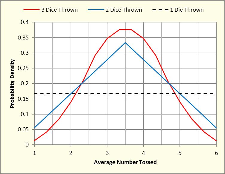
Figure 1. Comparison of average-value PDFs for tossing 1, 2, and 3 dice shows progression from uniform toward Gaussian probability density as the number of dice averaged increases.
The Central Limit Theorem goes on to explain: When N samples are taken from a population of mean μ and variance σ2 the mean of the average converges on μ, while the variance of the average approaches σ2/N. This means if you are offered a chance to gamble on the sum of 10 dice thrown together, always bet on 35. If the challenge involves 100 dice, bet on 350 and make your wager times as large. But what, you now ask does all this gaming have to do with random shake tests? That answer was provided by Dr. Athanasios Papoulis (1921-2002), a professor of electrical engineering at Brooklyn Polytechnic University.
In his 1962 book, The Fourier Integral and its Applications, Papoulis discussed the probability distribution of a narrow bandpass filter’s input and output. His analytic derivation recognized that the Central Limit Theorem applied exactly to this situation since the act of filtering can be recognized as a convolution. In turn, convolution can be recognized as a form of weighted averaging using the impulse response of the filter as the weighting function. This allowed him to make a very important observation: When a broadband random signal of almost any probability distribution is the input to a narrow bandpass filter, the probability distribution of the filter’s output approaches Gaussian. This statement is often called the Papoulis Rule. As we will find shortly, the words “narrow” and “approach” are quite significant to our accelerated life testing application.
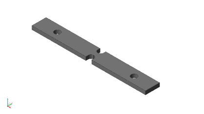
Figure 2. VRC standardized 6016- T651 aluminum notched-beam specimen (nominally 4 x 0.5 x 0.125 inch) fabricated in quantity to study fatigue. In use, one hole mounts beam to shaker, while the other mounts standard tip mass. Intended fatigue failure area is between symmetric round-end notches.
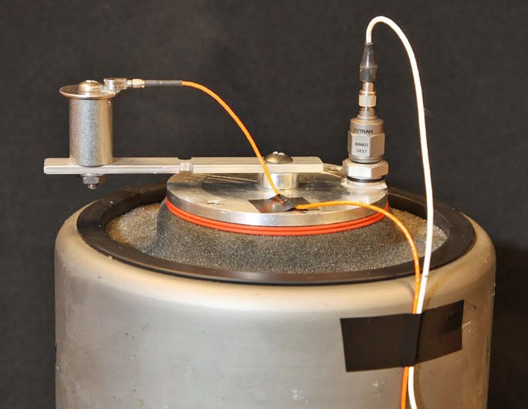
Figure 3. Testing notched beam on a small shaker. Accelerometer (right) mounted on shaker table measures the Control. Cylinder on left is standardized 50-gram mass. Small accelerometer mounted on this mass monitors beam’s free-end motion.
The Papoulis Rule
Vibration Research fabricated hundreds of standardized notched cantilever beams (see Figure 2) to provide a simple and repeatable target from which to gather fatigue statistics. Figure 3 shows a typical test. The beam is held to a shaker by a single bolt through either of its two holes and a spacer. A 50-gram mass is screw-mounted to the other hole. The Control accelerometer is mounted rigidly to the shaker table and a second (smaller) accelerometer monitors the motion of the mass.
The beam was subjected to a NAVMAT profile test controlled by a Vibration Research VR9500 controller. The kurtosis for this test was set to 9, a very high value. However, the transition frequency, a random control parameter unique to the VRC Kurtosion® process, was deliberately set to a high value. This was done so that the VR9500 would produce control results similar to those of alternative technology kurtosis control algorithms, including those predicated upon polynomial transformation and/or phase selection. Figure 4 presents a very interesting look at the probability distributions at the shaker head (cantilever beam root) and at the (weighted) beam’s free end. The figure is plotted with a logarithmic vertical axis, allowing a more detailed look at the high-excursion tails of the PDFs.
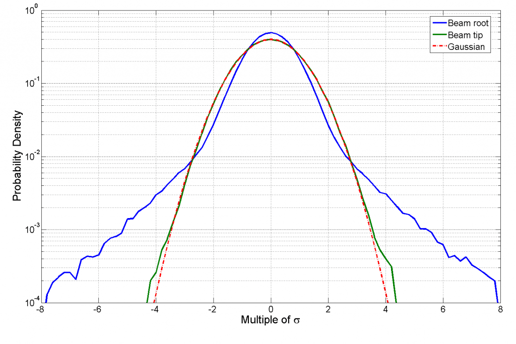
Figure 4. Normalized PDF of shaker head acceleration and cantilever root (blue), weighted cantilever free-end (green), and reference Gaussian distribution (red).
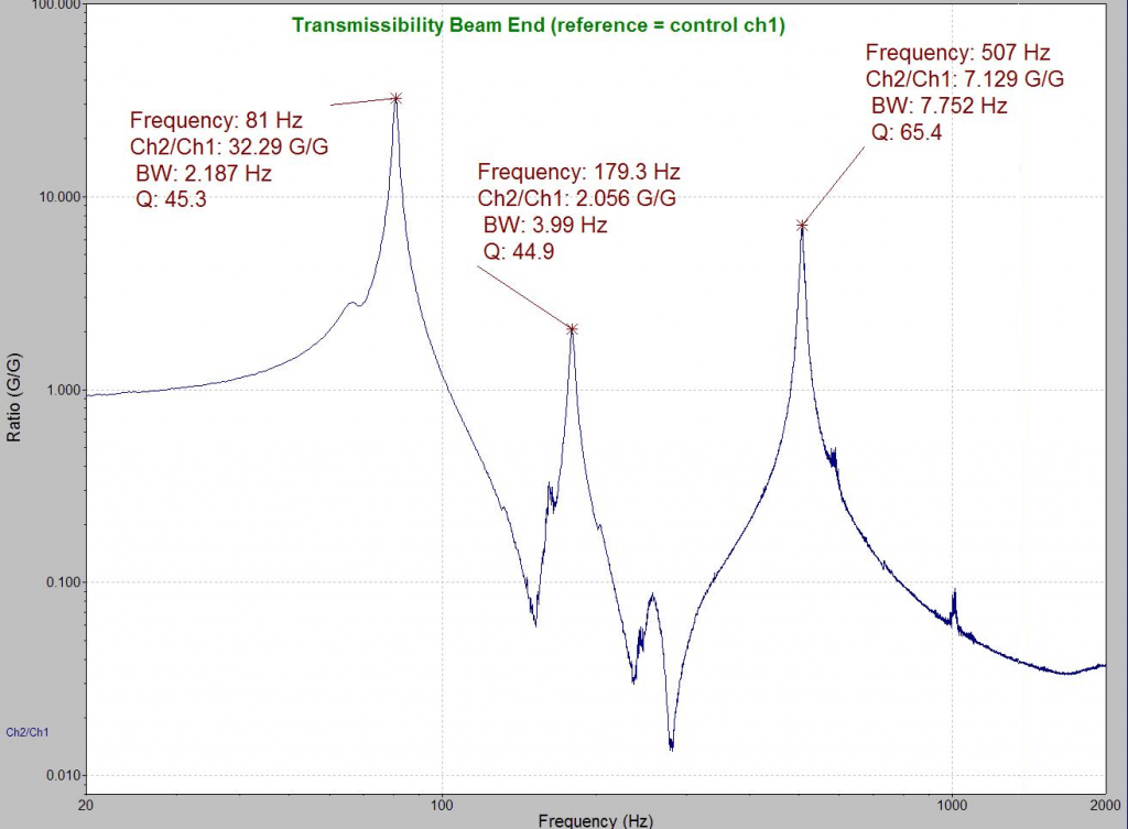
Figure 5. Cantilever tip/root transmissibility measured during NAVMAT PDF comparison test. Weighted beam’s dynamics are dominated by three high-Q modes of vibration occurring at about 81, 179, and 507 Hz.
The shaker table (blue trace) in Figure 4 has clearly wider tails than the reference (red) Gaussian distribution. This is the direct and desired result of specifying a high kurtosis of 9 for the test’s Control signal. However, the freely vibrating tip of the beam (green trace) exhibits an almost perfect Gaussian shape, indicating that it is experiencing a kurtosis of 3, not 9. The difference between these shapes and kurtosis values is entirely explained by the Papoulis Rule and has been used (misguidedly) by some competitors in an attempt to devalue the merits of high-kurtosis life testing.
As shown in Figure 5, three vibratory modes dominate the response of the weighted cantilever beam. These occur at nominal frequencies of 81, 179, and 507 Hz. Figure 5 shows that these mechanical resonances act like mechanical filters, restricting the bandwidth of the tip response to be dominated by these three frequencies. The NAVMAT test specifies a 6 gRMS random shake with a constant power spectral density (PSD) of 0.04 g2/Hz between 80 and 350 Hz. Above and below these extremes, the drive excitation diminishes at 6 dB/octave. Therefore, the 81 and 179 Hz modes are excited by the full intensity of NAVMAT’s central band, while the 507 Hz mode only receives about 65% of this stimulation. The tip response is clearly dominated by these three resonances, with the 81 Hz mode component more than 10 times as large as the other two modes. Therefore, these narrow-band resonances serve to filter the frequency content and reduce the kurtosis of the tip response to a Gaussian level in accordance with the Papoulis Rule.
Papoulis-Guided Accelerated Life Test
The Papoulis Rule contains two keywords of major import, often misinterpreted: approach and narrow. The rule does not say the output of a band-limiting filter will be Gaussian, it says the response approaches Gaussian. How rapidly that approach is made we now know is signal dependent. Kurtosion has a process-basic parameter that can be adjusted to ward off that approach, and we can now disclose it. To aid in industry acceptance of this innovative testing method, rather than simply keeping it a trade secret, we have opted for the much more expensive path of patent protection so that we can reveal the inner details while still protecting our legal rights. With the issuance of U.S. Patent 7,426,426 B2, System and Method for Simultaneously Controlling Spectrum and Kurtosis of a Random Vibration, we can now candidly discuss the details of Kurtosion.
Kurtosion generates high-kurtosis random signals through a modulation process. First, a Gaussian white noise signal is generated, and this is amplitude modulated by a second random noise. The signal specifics of this second random signal determine the kurtosis of the result, which is then frequency shaped by the desired Demand and the measured H–1 frequency response of the shaker/amplifier/DUT electromechanical system. One of the detailed parameters of this process is the lower frequency corner of the modulation process’s bandwidth. We have chosen to call this parameter the transition frequency, and it is a user-specified parameter of a test.
The rules for setting the transition frequency are quite simple. Measure the transmissibility of the DUT (Figure 5, for example) and extract the bandwidth (BW) frequency of each resonance within the frequency range of the test. Set the transition frequency to be less than the BW of any dominating resonances, as shown in Figure 6. Now run the high-kurtosis test.
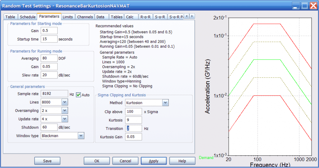
Figure 6. Setup dialog for high kurtosis random test showing entry of transition frequency
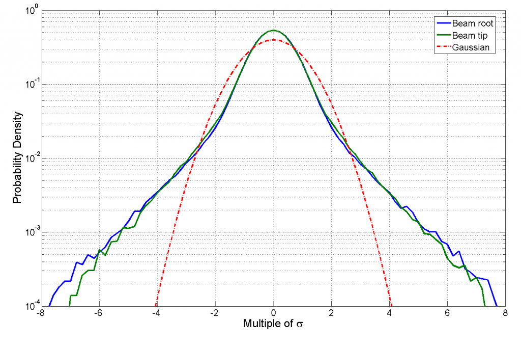
Figure 7. Figure 4 with transition frequency set less than BW of all modes in test frequency span. Both root and tip of beam now show high kurtosis far exceeding the Gaussian model in their PDF tails.
Figure 7 shows the result of such actions. The test previously illustrated is repeated, but this time the Transition frequency is set to less than the BW of the narrowest of three vibration modes, rather than being deliberately greater as it was in Figure 4. Note that both the tip and root of the cantilever beam now exhibit high (and essentially identical) kurtosis far in excess of the Gaussian model. This is shown by the wide skirts or “tails” of both the blue and green traces. The only difference between the test conditions of Figures 4 and 7 was the transition frequency setting.
Early in our development of Kurtosion, we became interested in verifying that the programmed kurtosis was applied equally across the entire bandwidth of the control signal. We used a bank of standard 1/3-octave filters to examine this. The control signal was filtered by the 1/3-octave bank, and the kurtosis of each filter’s output was computed. When plotted as a kurtosis-versus-frequency spectrum (Figure 8), this test gave the false impression that controlling kurtosis to a value greater than 3 was difficult at a low frequency. Recall that each filter in a 1/3-octave set has a half-power (–3 dB) bandwidth equal to 23.1% of the center frequency of that filter. Actually, it was the narrow bandwidth of the low-frequency filters that caused the kurtosis to decline at low frequency, not the center frequency of those filters. In other words, we saw an early demonstration of the Papoulis rule but initially failed to recognize it. As in so many human endeavors, wisdom in the control field comes only with continued effort and study.
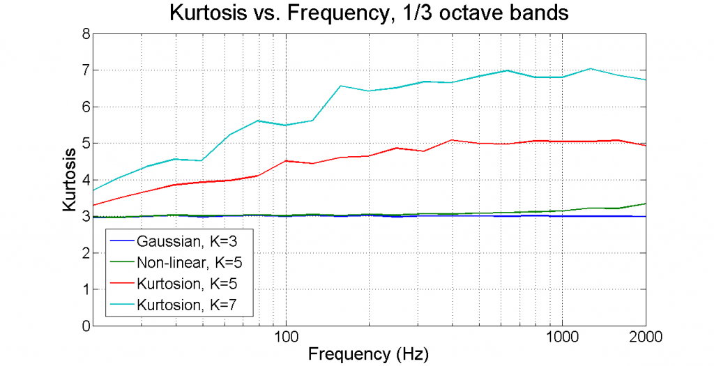
Figure 8. Early VRC kurtosis-versus-frequency plot made using 1/3-octave filters suggests low-frequency kurtosis greater than 3 is difficult to achieve – an erroneous conclusion.
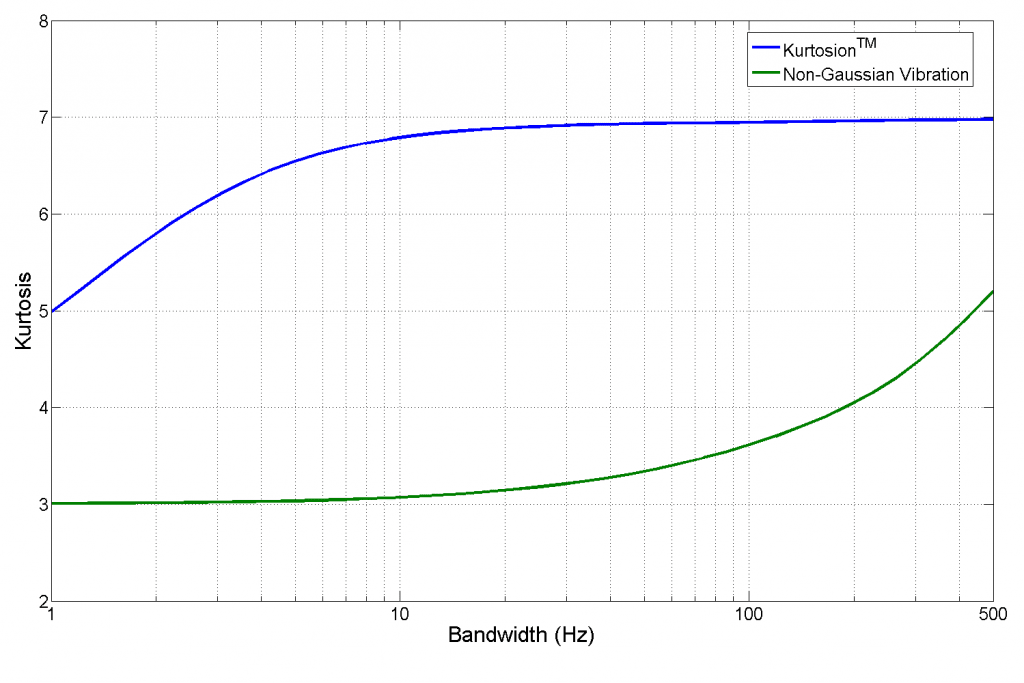
Figure 9. Comparison of measured filter output kurtosis at 300 Hz for filters of 1-500 Hz bandwidth all exposed to identical NAVMAT profiles with controlled kurtosis of 7 (blue = kurtosion with 2 Hz transition; green = non-Kurtosion control).
Figure 9 illustrates the application of a rather different filter bank to two signals matching the NAVMAT profile of Figure 6. Both traces in Figure 9 used an excitation signal with a measured and controlled kurtosis of 7. The blue trace was generated using Kurtosion with a transition frequency of 2 Hz, while the green trace presents high-kurtosis control with a transition frequency of 4000 Hz (equivalent to a signal created using the polynomial transformation technique). Both signals were passed through a bank of second-order resonant response filters all centered at 300 Hz but with the bandwidth of the response peak varied from 1 to 500 Hz. The kurtosis measurements of the filters’ outputs were plotted to form a kurtosis-versus-bandwidth spectrum.
Note that the blue signal with the low transition frequency maintains the full kurtosis of the source signal through resonant responses with bandwidths as low as 10 Hz. Below 10 Hz, the kurtosis begins to fall off, although it maintains a kurtosis of 5 even with a bandwidth of only 1 Hz. In contrast, the green signal with the high transition frequency fails to maintain the kurtosis level of the excitation signal even at a 500-Hz bandwidth and is indistinguishable from Gaussian for any bandwidth less than 10 Hz. As the bandwidth approaches 0, the filter output tends toward Gaussian as predicted by the Papoulis Rule. However, by using a properly constructed excitation signal, a respectable kurtosis can be maintained at the resonance for the bandwidths typically encountered in mechanical systems.
The results of Figure 9 can be roughly compared to our resonant beam tests. Note from Figure 5, that the 81-Hz first mode (the shape that failed in fatigue) had a bandwidth of about 2. Figure 9 illustrates that a signal generated using Kurtosion with a kurtosis of 7 and transition frequency of 2 Hz will induce a kurtosis level of nearly 6 at a 2 Hz wide resonance, while the signal lacking appropriate transition frequency control exhibited very slightly more than 3. Clearly, a high-kurtosis signal generated with a low transition frequency can pass through a narrow-band process to produce a (more damaging) high-kurtosis output.
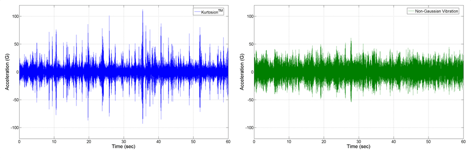
Figure 10. Comparison of monitored beam-tip signal for tests of Figures 4 and 7. Note more extreme excursion of the properly set Kurtosion (upper blue) signal than that of other control strategies for the same (k=9) setting.
Figure 10 provides a blatantly simple verification of the importance of the transition frequency. This plot compares beam-tip time-history samples from the tests of Figures 4 and 7. Note the more extreme excursions of the upper blue trace (Kurtosion with properly low transition frequency), despite both tests specifying kurtosis equal to 9. The deliberately high transition frequency of the lower trace prevents the resonances from being excited to the specified high-kurtosis level.
Clearly, kurtosis greater than 3 can be made to pass through a narrow-band filter or a mechanical resonance if proper care is given to its supporting metrics. That is, you can “get the kurtosis into a resonance.” We have established and demonstrated that setting the transition frequency of a Kurtosion test to a value less than the passband of the filter or band-limiting resonance is the key. This raises an obvious question: why not always set the transition frequency to the lowest possible value supported by the hardware/firmware/software? The answer is simple: this value is a trade-off with the responsiveness of the control loop. As the transition frequency is reduced, the high-energy events in the random signal become more separated in time. Unless the averaging degrees of freedom (DOF) is increased, the measured H–1 can become “short-term focused,” resulting in an up/down “bounce” in the Control signal. Therefore, the transition frequency, like the averaging DOF, is best left as a user choice allowing intelligent optimization of every test circumstance.
Experimental Demo of Accelerated Life Testing
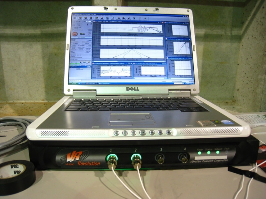
Figure 11. VR9500 Revolution controller runs multiple specimens to destruction using NAVMAT profile.
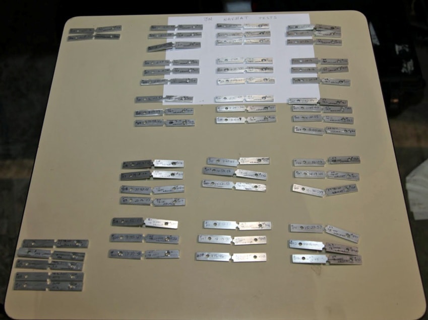
Figure 12. Fatigue specimens broken during this examination.
A large number of our standardized specimens were run to destruction using a NAVMAT random profile. These tests were managed by a VR9500 controller while running the Random software with Kurtosion. Multiple runs were made at kurtosis values of 3, 5, 7, and 9 using the control system illustrated in Figure 11. Typical specimen installation on the small PM shaker is shown in Figure 3.
All specimens tested eventually yielded and fractured at the center notch as anticipated. The controller measured the duration of exposure for each sample and notified the test engineer via email upon its failure. Multiple runs were made for each kurtosis setting, allowing the results to be spreadsheet averaged. Recognize that such data collection is a slow and methodical business. Runs made using a Gaussian distribution typically required more than a work shift to fail the specimen.
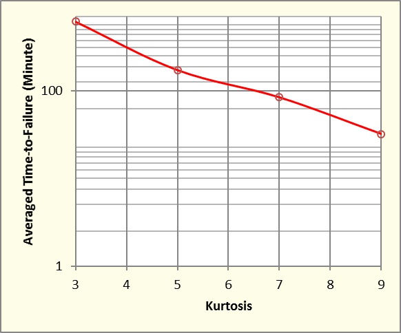
Figure 13. Average minutes to failure versus kurtosis of control signal.
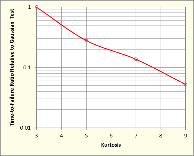
Figure 14. Average time to failure normalized to Gaussian failure time versus kurtosis of control signal.
Figure 13 illustrates the variation in averaged time to failure with kurtosis setting. As shown here, failure time decreases approximately exponentially with linear increase in kurtosis, suggesting a power law relationship. Bear in mind that all of these tests were conducted using exactly the same spectrum profile and RMS intensity. They differed only by the controlled kurtosis target.
Figure 14 presents the same results divided by the averaged failure time for a Gaussian control signal. Clearly, increased kurtosis accelerated fatigue failure of this simple resonant beam. Raising the kurtosis to 5 dropped the required failure time to 28% of that required for a Gaussian control. A kurtosis of 7 cut this in half again to 14%, while setting the kurtosis to 9 broke sample beams in about 5% of the time required at kurtosis equal to 3.
Conclusions
We have demonstrated that increasing the kurtosis of a random signal above the Gaussian value of 3 can increase the damage-inducing potential of the profile. We have further debunked the old wives’ tale that increased kurtosis cannot influence the fatigue accumulated by a structure with resonances within the band of a random test.
We have shown by example that a general-application broadband profile (such as NAVMAT) can be used to identify fatigue-sensitive resonances and that such testing can be accelerated in time by increasing the kurtosis of the controlled shake. To this end, we have shown that while the Papoulis Rule shows that narrow-band filtered signals tend toward a Gaussian distribution, not all signals with the same kurtosis are created equal. Some signals succumb more readily than others. With the flexibility of the transition frequency parameter in our patented Kurtosion testing method, you can easily create waveforms that allow increased kurtosis to pass into the resonances of your product.